How I Learned Atari from Pixels with Deep Q‑Learning

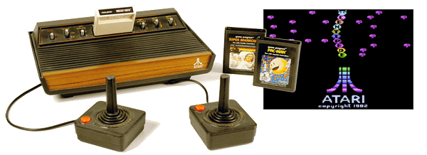
Today we are brainstorming the 2013 paper, “Playing Atari with Deep Reinforcement Learning” by DeepMind Technologies. This paper was published about one month before Google announced it would acquire DeepMind in January 2014.

Why this paper still matters

Why are we talking about this 2013 paper?

This paper still matters because it was the first to demonstrate that a single convolutional neural network trained with Q‑learning can learn control policies directly from raw pixels across multiple Atari games without game‑specific features, reaching and surpassing human performance on some titles. It also established a practical training recipe:

experience replay, stacked frames, reward clipping, and consistent architecture

that remains the conceptual baseline for deep reinforcement learning today. This also makes this algo much more general than the previous ones.

Around 2013, all deep learning applications required large amounts of hand-labelled training data.

The challenge in plain words

• High-dimensional input: ~7,000 pixels per frame (after downsampling) × 4 frames.

• Partial observability: A single frame misses velocity; hence the 4-frame stack.

• Sparse and delayed rewards: Many games don’t reward you every frame

• Strong generalization ask:

  • One network architecture should learn diverse games

  • the only thing different between games is the action space

Reinforcement Learning

Before we begin, lets quickly go over the most general framework in which most RL problems are constructed.

An agent interacts with the environment in a sequence of actions, observations and rewards.

State -> snapshot of environment
Action -> decision taken by agent in an environment

3 signals passed between the Agent and the Environment:

• State: environment’s way of presenting a situation to the agent

• Action: agent’s response to the state. It influences the environment

• Reward: environment’s response to action, giving some indication to the agent about the correctness of its action.

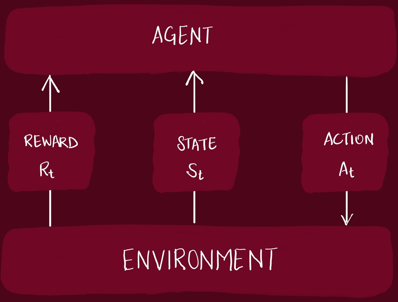
At each step, the Agent selects an action from the set of legal actions allowed. The action is passed to the environment, which modifies the internal state in someway.

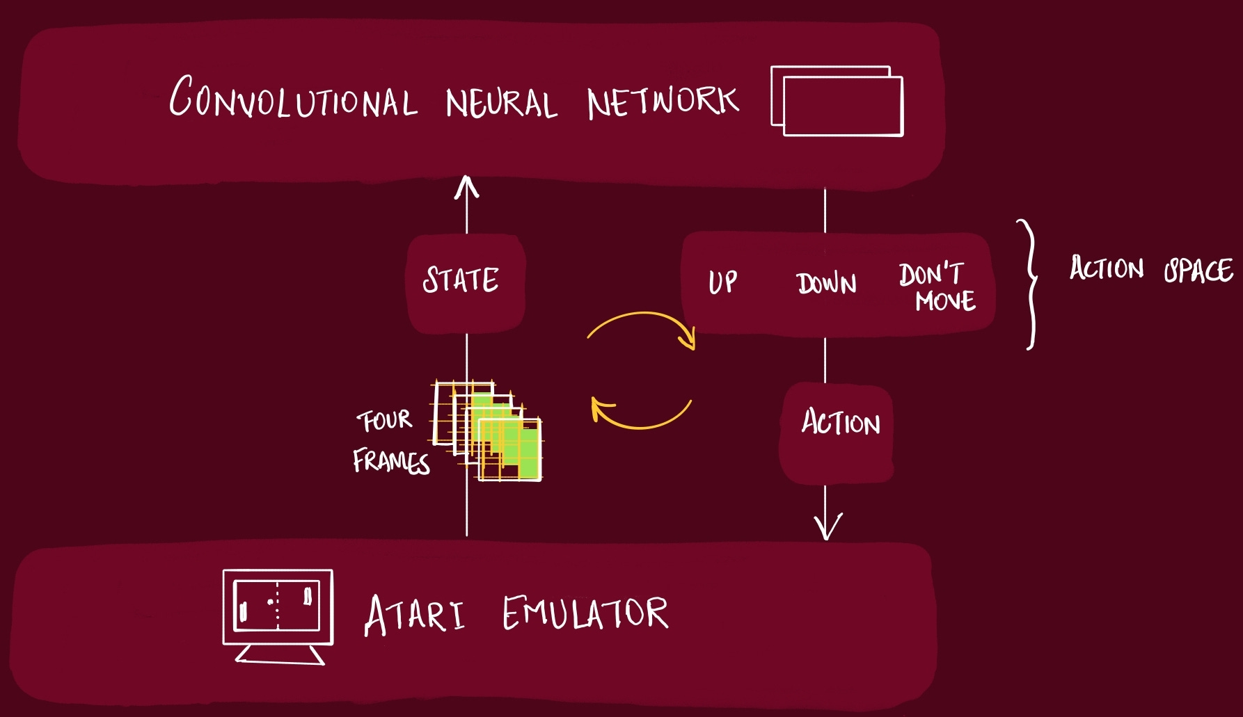
In this paper, the experiment that the authors have setup, the Agent can only access a vector of raw pixel values representing the current screen. When the Agent does an action, it receives a reward, representing the change in game score.

In this paper, the CNN is the Agent.

If you have played any video-game, you know the reward comes after playing it for a few moves. The reward is sparse, delayed, and not guaranteed at all.

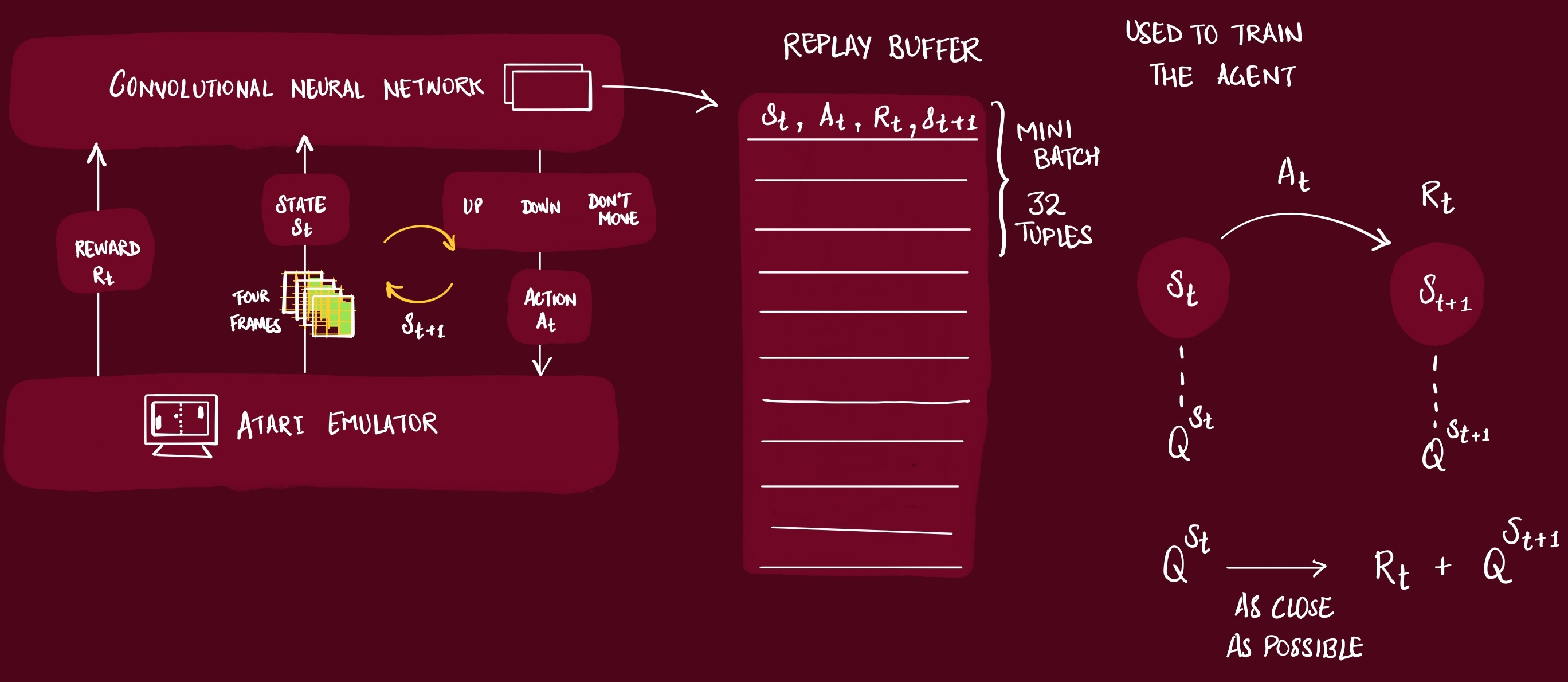
As the Agent plays the game, the information is captured in a Replay Buffer. This buffer is later used to actually train the Agent. What we actually store in this buffer is:

[state, action, reward, next state]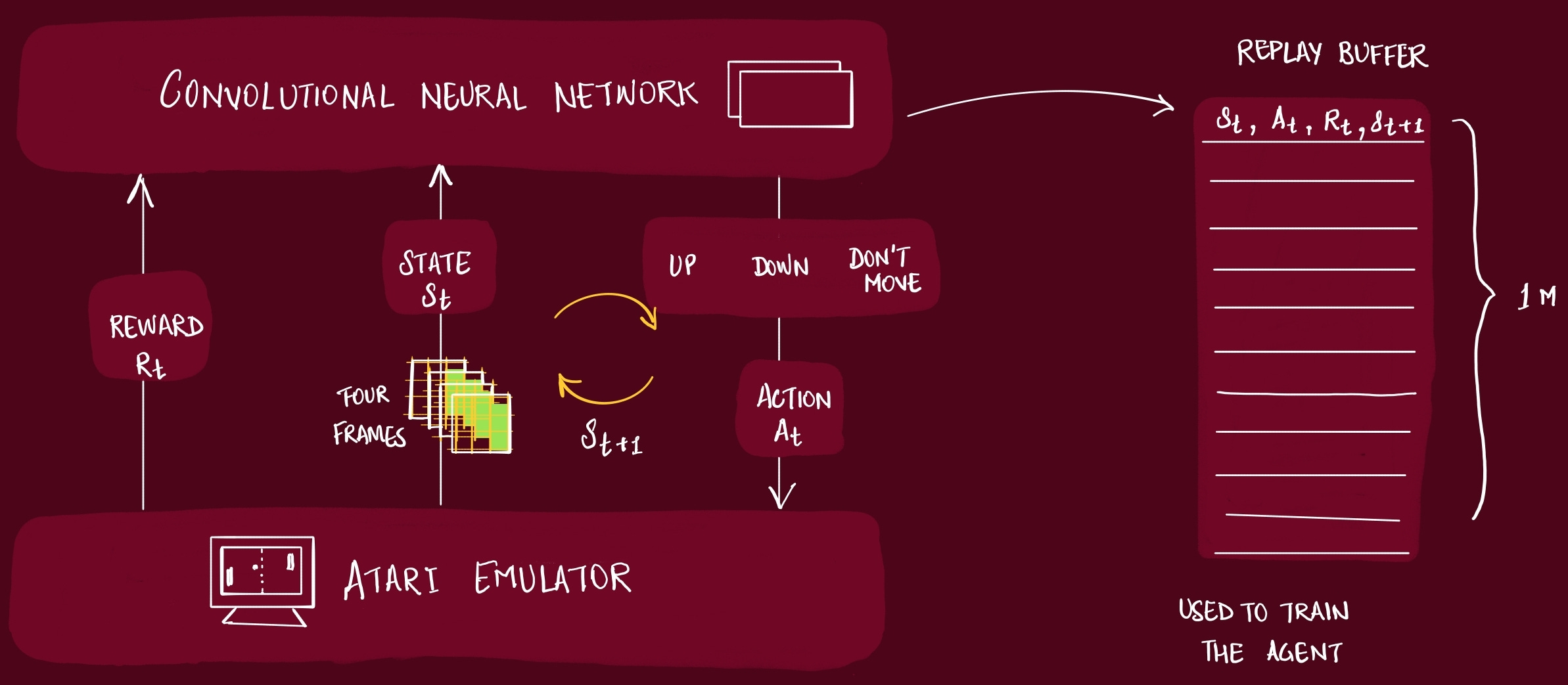

Actions have short and long-term consequences and the agent needs to gain some understanding of the complex effects its actions have on the environment.

Since the previous Rewards (generated from previous actions) is already known, the Agent tries to maximize the Cumulative Future Rewards.

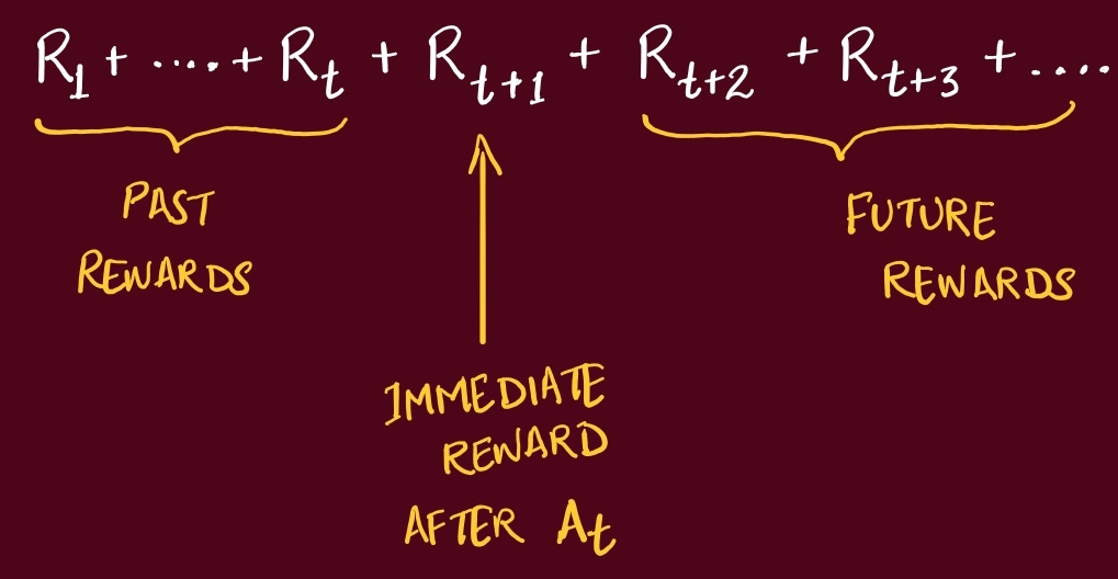
Remember, the goal is always to maximize the Cumulative Reward.

But it’s very difficult for the Agent to differentiate near future reward expectation vs rewards that might come in 20 or 50 steps later.

\(R_{t+2} ----- R_{t+20}\)

So, it makes sense to allocate more value to rewards which are closer to Agent, compared to rewards which would happen in future.

We need a technique so the agent doesn’t have to think too far into the future.

This is referred to as Discounted Return. This way we have a nice decay where rewards earlier in time are always multiplied by a larger number, indicating the agent to prioritize them.

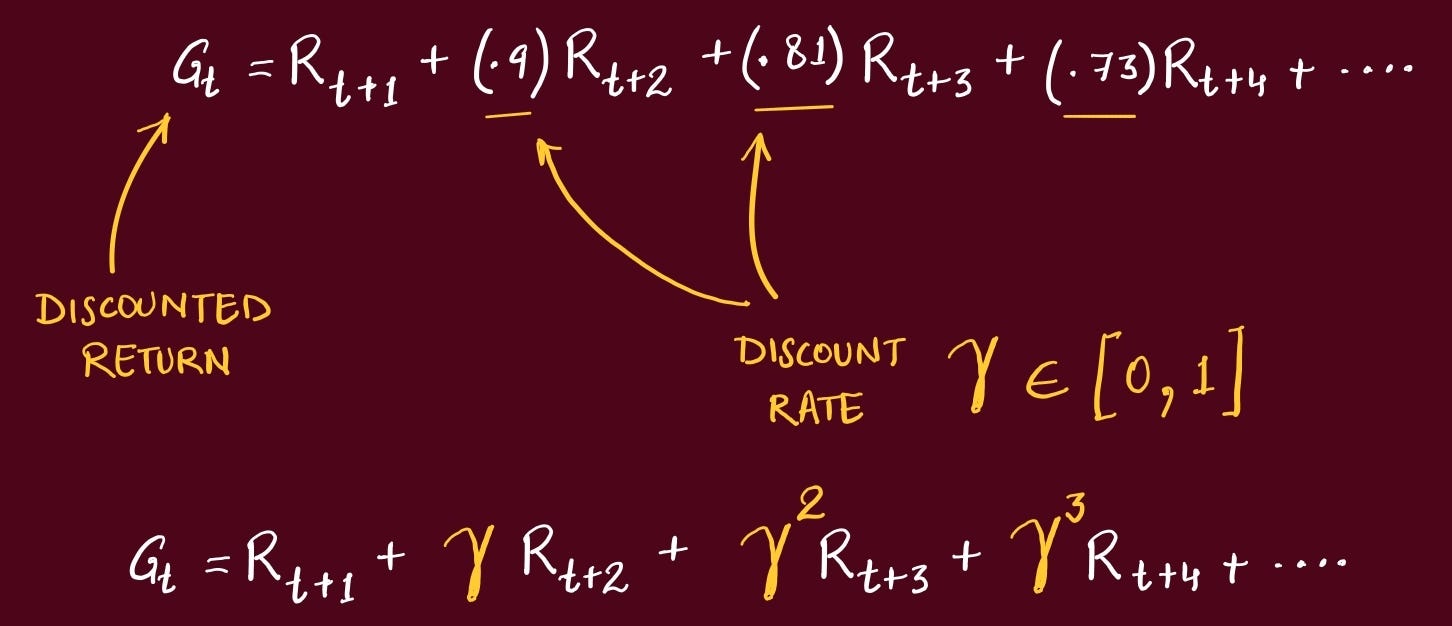
The Gamma is set by us, based on our goals for the agent.

The larger you make Gamma, the more the agent cares about the Future.

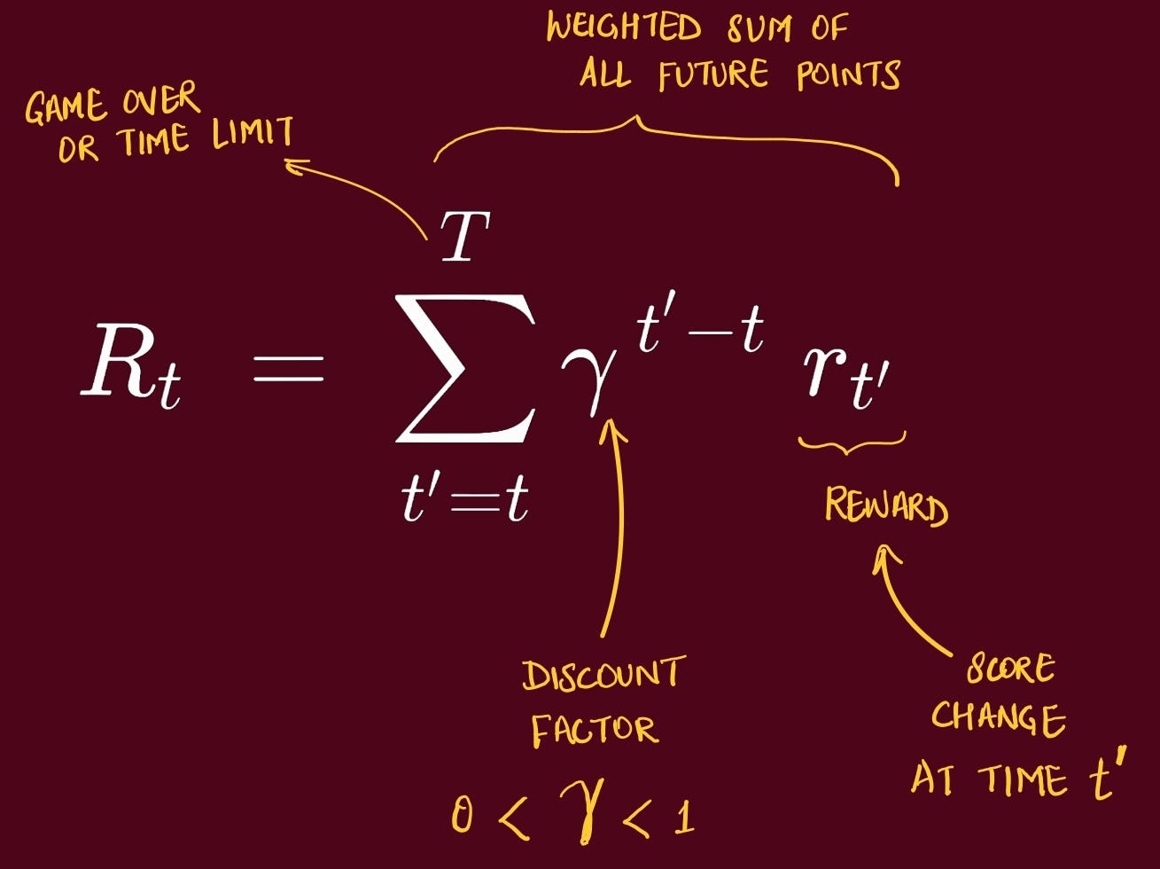
In this paper, the exact quantity the agent tries to maximize is, starting at time t, the discounted return:

Q-Learning

This is one of the most important topics from Reinforcement Learning (RL).

Policy -> is how an agent behaves in a given situation.

Broadly RL algorithms can be divided into 2 types:

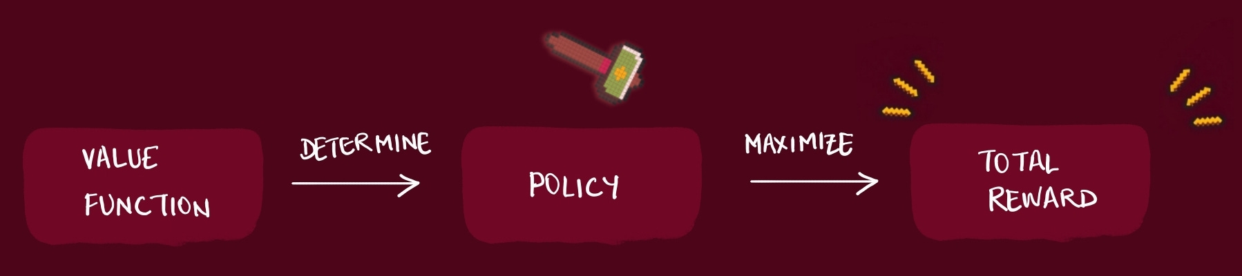
1. Value-based methods

   1. determines a value function → that quantifies the total reward.

   2. this is used to then decide the optimal policy

2. Policy-based methods

   1. determines an optimal policy directly → maximizes total reward.

Q-Learning is a Value-based RL method.

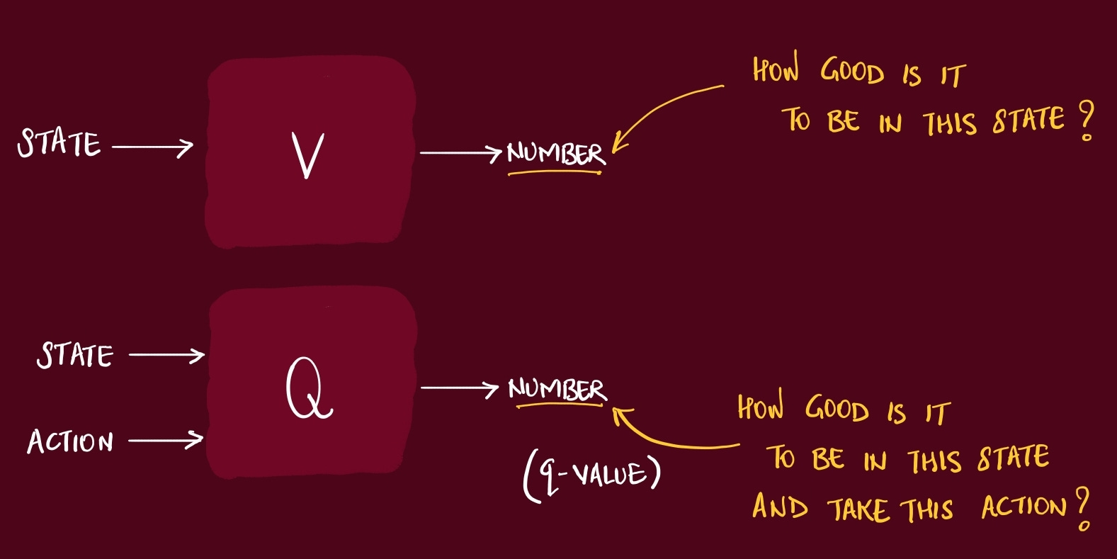
Since Value function is a function (input & output), based on it’s input, there are 2 types of Value function:

1. State Value Functions V(s)

2. State-Action Value Functions Q(s, a)

We can compare these two functions as below. Both functions generate a numeric output which is some indication of how good current state or taking an action is.

To easily visualize this, imagine a table with all combinations of States and Actions. Each cell is then the Q value of that State + Action.

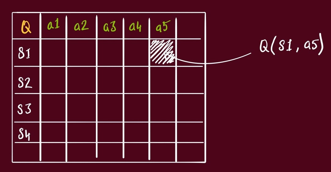
This is very traditional way of looking at scenarios, because if you imagine any scenario, you would realize this table would have

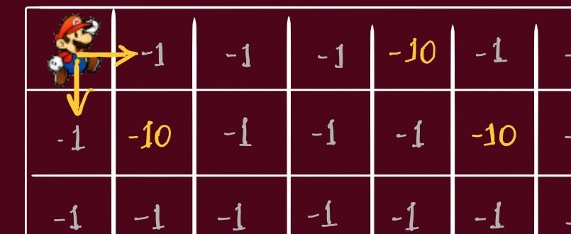
Take an example of my favorite childhood game.

The hero has to move from it’s original state to final state, collect all powerups, avoid danger, and do so in least possible steps.

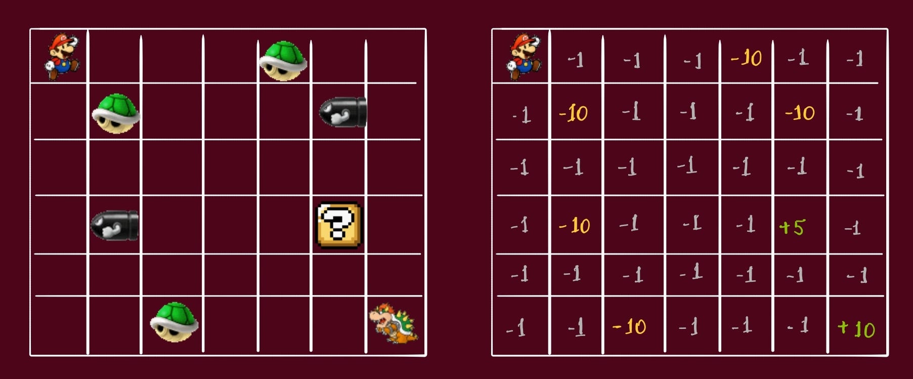
We can see the same game on the grid:

• things to avoid = -10

• power-ups = +5

• final destination = +10

• all others = -1

We want the character (agent) to learn an optimal policy, or Target Policy. We start with by initializing this table with arbitrary values.

Key point: This table could also be loaded by some other agent that has previously explored the environment.

Initially, the character (agent) is just exploring. At this state, the character (agent) can go either right or down. Since, the behavior policy is random, we can assume the agent goes to right.

When the agent goes right

• it’s now in State = S2

• received a Rewards of -1

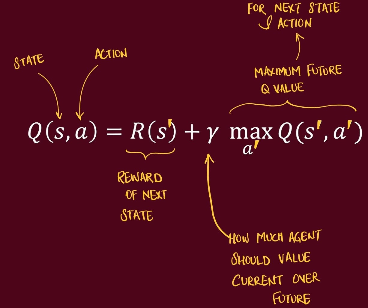
The relationship between states is calculated using Bellman Equation. It gives us the observed Q value at S2:

Deep Q-Learning (DQN)

DQN learns a function Q(s,a) that estimates the expected discounted return Rt if you take action a now in state s and then act optimally thereafter. When the agent picks an action, it chooses the one with the largest estimated Q

the one that leads to the highest expected sum of discounted future rewards.

Randomly initialized -> a state is choosen -> Agent chooses an Action -> Action is performed -> Reward is gained -> Agent goes to next state

With each action, we store the information in Experience Replay Buffer

[S1, right, -1 S2]
[S2, right, -1 S3]
....
[S4, right, -10 S5]

In DQN, we have two phases:

• Data Collection Phase

  • randomly initialize q-network (NN)

    • number of nodes in output layer = number of possible actions

      

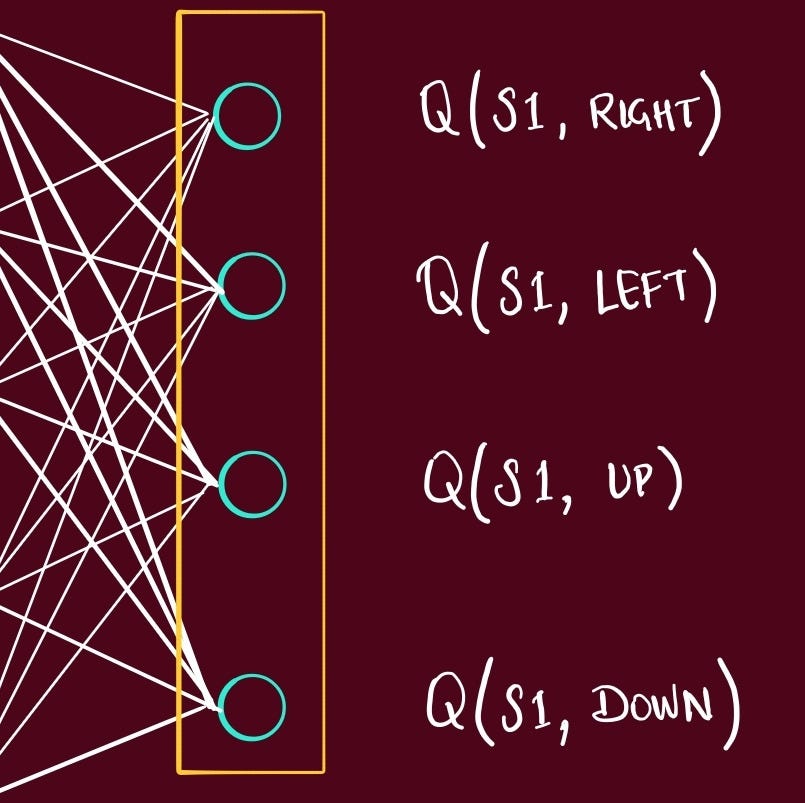
  • choose initial state

  • pass it through q-network (NN)

  • generates a Q value → corresponding to each action

  • action is picked (greedy)

  • action is performed

  • agent gets reward

• Training Phase

  • For an action, state

    • Q-value is calculated for q-network = Qn

    • Q-value is calculated for Target network = Qt

      • we add the reward to this, Qt + R = Qtr

  • Compare

    • Mean Squared Error (Qn, Qtr) = E

  • This is back propagated into the q-network, parameters are updated

  • q-network learns, target network remains same

Target network - iteration in the direction of ideal. it gets updated after few batches.

MDP

A Markov Decision Process (MDP) is a clean blueprint for making good choices when outcomes are uncertain and unfold over time.

Picture a robot in a maze: at each square (the state) it chooses a move (the action), then the maze “responds” by moving the robot to a new square and giving it a reward (good or bad points). The robot wants a strategy (a policy) that maximizes its long-term points. The Markov bit says: what happens next depends only on where you are now and what you do now, not on the entire past.

MDP:

• where you can be (states),

• what you can do (actions),

• how the world reacts (transition probabilities and rewards), and

• how much you care about the future (a discount).

We model Atari as an MDP:

• large but finite Markov decision process (MDP) in which each sequence is a distinct state

• goal of the agent is to interact with the emulator by selecting actions in a way that maximises future rewards

The training loop

As we already discussed, when the Agent walks through the game, each timestep collects a transition, and stores it in replay buffer. We then sample a random minibatch of 32 size from this buffer, and use it to train the Agent.

The states stored in the replay buffer are used to train the agent.

Simply, they pick a stack (4 frames), take max q-value of each state → Sum them up → take the average → only store the max q-value of all these state.

Core ideas

1. End-to-End Pixels-to-Actions Learning

   1. What the agent “sees” and does

      1. agent interacts with an environment E (the Atari emulator) in a sequence of actions, observations, and rewards.

      2. At each time-step t

         1. it picks a legal action a ∈ {1,…,K}

         2. receives a screen image x (raw pixels)

         3. and a reward r​ (change in game score)

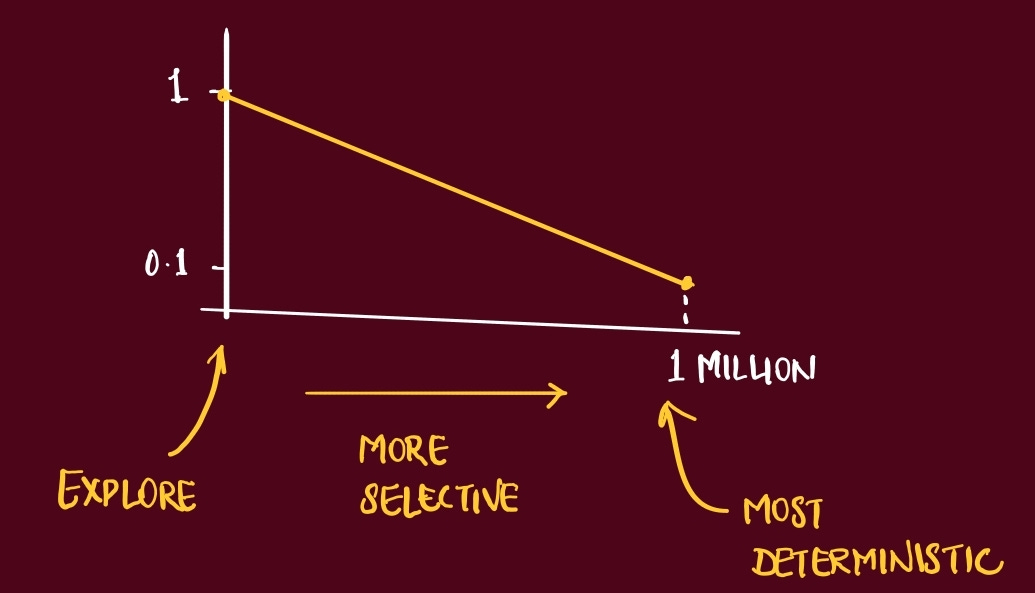
      3. action at each step is selected via an ε-greedy policy during training

         1. making the exploration mechanism explicit in the core loop description

         2. ε (epsilon) → probability of taking a random action

         3. ε starts high (e.g., 1.0) to encourage exploration, and is gradually reduced (annealed) to a lower value (e.g., 0.1) over time

         4. guarantees the agent sees enough of the world early on and doesn’t stop exploring too soon

            

   2. Because the agent can only see the screen (pixels)

      1. at any given time, the task is only partially observed if you look at the current state

      2. consider sequences of actions and observations, State = x1, a1, x2, a2...

         

   3. Think of the agent like a novice player

      1. who only sees the screen and feels the score.

      2. learns which joystick move tends to raise future points

      3. mapping pixels → value estimates → actions

   4. Temporal State via 4-Frame Stacks (84×84×4)

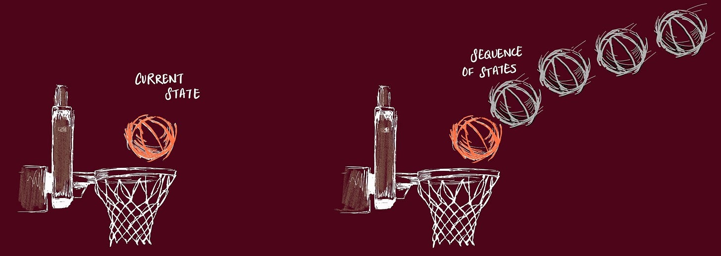
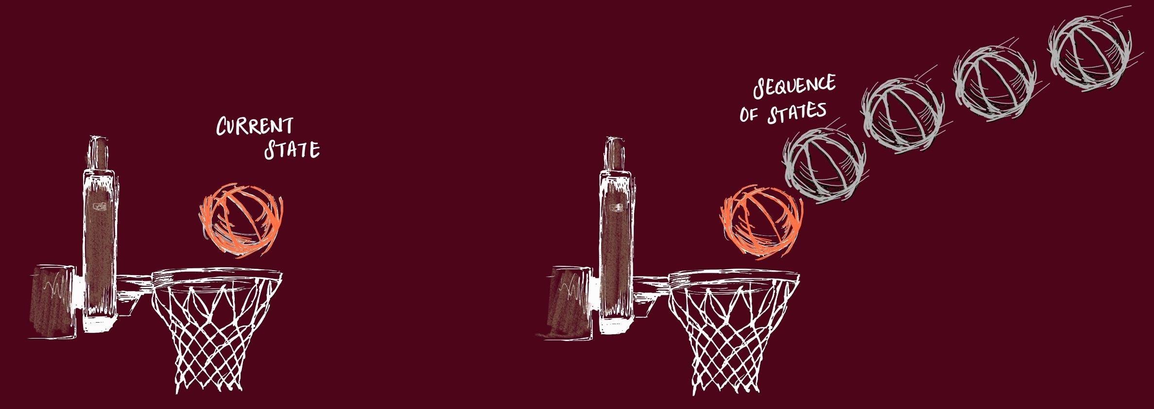
      1. If you freeze a single Atari frame, a lot is missing

         1. velocity and direction are hidden

      2. The ball is just a dot → no hint of whether it’s racing left or right

      3. Stack 4 frames in time order

         1. RL algorithms work best when the “state” contains enough information to predict what happens next

         2. last 4 preprocessed frames

         3. from this, a CNN can infer motion

            1. e.g., “the ball moved +3 px right, −2 px up per frame”

            2. which is exactly the clue you need to place the paddle

      4. What exactly goes into the stack

         1. Gray scale - Collapse RGB to a single channel to cut input size and keep the signal clean.

         2. Downsample + crop to 84×84. Standardize resolution across all games

         3. ~28k numbers (4×84×84) per state

            1. small enough for fast training, rich enough for short-term dynamics

2. Experience Replay as a Stability & Data-Efficiency Engine

   1. Imagine trying to learn pool by only practicing the last shot you took, over and over.

      1. You’d get really good at that one shot,

      2. but your overall game would stall, and

      3. every tiny habit you pick up would instantly echo back into your next attempt.

   2. What this paper does:

      1. Keep a replay buffer of past transitions

         1. [state, action, reward, next state]

         2. 1 Millions array slots

      2. Instead of learning from the latest step, sample random mini-batches from this buffer.

      3. Minibatch optimization

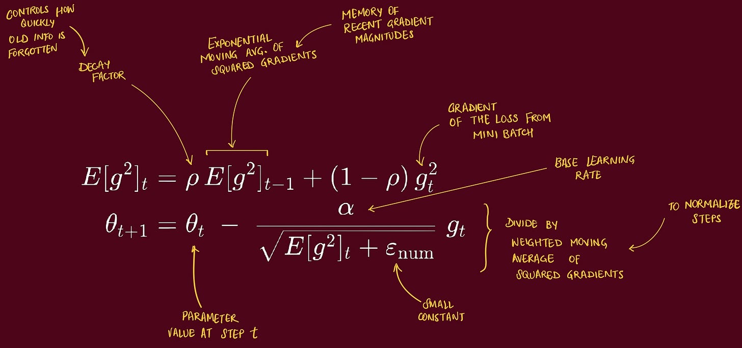
         1. sampled transitions are used to perform gradient steps with RMSProp (batch size 32)

            1. RMSProp (Root Mean Square Propagation) is an adaptive learning rate optimization algorithm

               1. used to train deep NN efficiently → when gradients can vary a lot across parameters or over time (zig-zag)

                  1. because all parameters share one global learning rate

               2. adapts the step size independently for each parameter

                  1. by keeping a running average of recent squared gradients

                  2. Parameters with large gradients → get a smaller step

                  3. calm parameters → get a larger step

                  

   3. Why was this done

      1. De-correlation. Shuffling breaks the “all from the same moment” pattern

      2. Smoothing the behavior distribution. You’re training on a mixture of older and newer policy behaviors, not just the current one

3. One CNN to Play Them All

   1. The model is deliberately tiny so it runs fast and generalizes

      Input:  (4, 84, 84)     # 4 stacked grayscale frames
      Conv1:  16 filters, 8×8, stride 4, ReLU
      Conv2:  32 filters, 4×4, stride 2, ReLU
      Fully Connected Hidden Layer:     256 units, ReLU
      Head:   |A| linear outputs (one Q-value per legal action)

   2. single forward pass returns all action-values at once

      1. so picking an action is just argmax over that output vector

   3. The only game-specific piece is |A|

      1. the number of legal actions

      2. everything else (layers, sizes, ReLUs) stays identical across games

   4. Reward Clipping

      1. reduce game rewards into {−1, 0, +1}

      2. keeps learning numerically stable across games with wildly different scoring systems

   5. Action repeat / frame-skip

      1. Paper uses a simple frame-skipping technique

         1. agent sees and selects actions on every kth frame instead of every frame

         2. its last action is repeated on skipped frames

      2. commonly k=4, with a small exception like k=3 in Space Invaders :)

      3. reduces flicker and speeds training by focusing on meaningful changes

4. Evaluation & Results: Beating Baselines and Humans

   1. How do you fairly score an agent that claims to “learn from pixels” across very different Atari games?

   2. The paper was also made possible thanks to the The Arcade Learning Environment (ALE), released a year prior

      1. which provides an evaluation methodology and toolkit for testing RL agents in Atari games

   3. ALE provides an evaluation set built on top of the Stella an Atari emulator

Experiments

Like we talked before, the only change to reward structure of the games during training, was Reward Clipping.

reduce game rewards into a scale of {−1, 0, +1}

This allowed them to use same set of hyperparameters across games, since the agent cannot differentiate between rewards of different magnitude.

Results

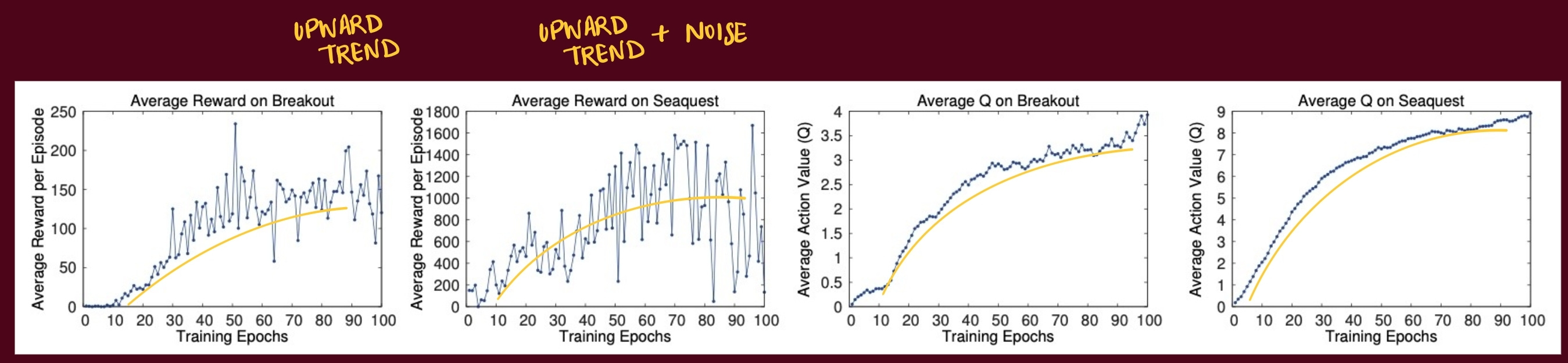
The metrics that the authors choose is the Average Q value. They collected a fixed set of states by running a random policy before training starts and track the average of the maximum predicted Q for these states.

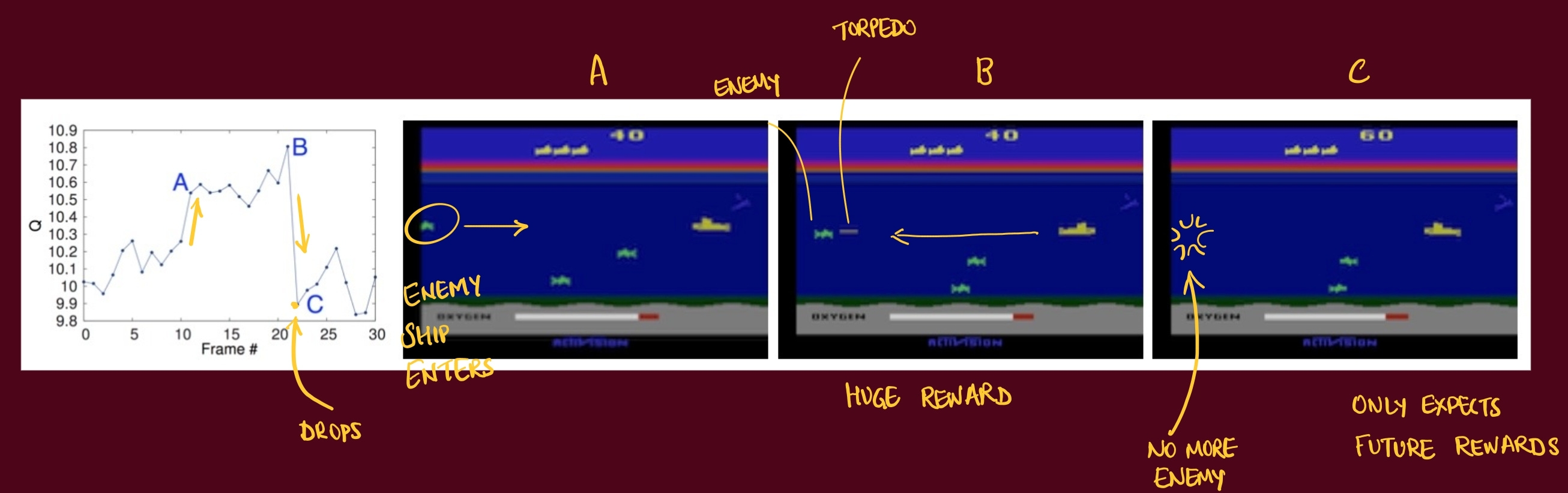
Dissecting a scene

Adapt it beyond Atari

Coming soon..